Understanding Bill Gosper's continued fraction arithmetic (implemented in Python)

Continued fractions are very often said to be the most natural or elegant way for representing numbers. Imagine a parallel universe, in which continued fractions are used as the dominant number system. People there use continued fractions for everything. So you'd think they calculate with them, too. But can you calculate with continued fractions? Most presentations on this subject don't talk about arithmetic at all. This gives the impression that you can't really do anything with them, except for looking for patterns in the coefficients when they are used to represent irrational numbers.

In fact, in 1972, mathematician and computer scientist Bill Gosper developed an ingenious method for doing exact arithmetic on continued fractions. Unfortunately, this method was published as an informal memo, which left out many details. I decided to implement the main idea in Python, and explain the reasoning in my own way. You can find Gosper original memo and additional information here. The source code is available here.

Since we'll use rational numbers a lot, let's define a class:

class Rational(NamedTuple('Rational', [('a', int), ('b', int)])):
    """Rational(a, b) = a/b"""
    def __repr__(self):
	return f'{self.a}/{self.b}'

How to convert a rational number to a continued fraction? Observing that

\[ \frac{254}{100} = 2 + \frac{54}{100} = 2 + \frac{1}{\frac{100}{54}} = 2 + \frac{1}{1 + \frac{46}{54}} = 2 + \frac{1}{1 + \frac{1}{\frac{46}{54}}} \]

it should be obvious that the solution is just the Euclidean algorithm for finding the greatest common divider: we first decompose the numerator \(a\) as \(a=b*q+r\), where \(b\) is the denominator, \(q\) is an integer called the quotient, and \(r\) is the remainder. We output \(q\), and repeat the process, using \(b\) as the numerator and \(r\) as the denominator. We stop when the numerator becomes 0.

# Convert a rational number to a continued fraction

def qr(a: int, b: int) -> Tuple[int, int]:
    """
    Find the quotient and remainder of a rational number.

    a = b * q + r, return (q, r).
    :param a: The numerator of the rational number
    :param b: The denominator of the rational number
    :return: (quotient, remainder)
    """
    q = math.floor(a / b)  # the quotient
    r = a - b * q          # the remainder
    return (q, r)

def r2cf_(rn: Rational) -> Iterator[Tuple[int, int]]:
    """
    Turn a rational number into a continued fraction.

    The Euclidean algoirthm.
    :param rn: The rational number
    :return: An iterator of the old denominator and the quotient
    """
    a, b = rn
    while True:
	q, r = qr(a, b)
	yield b, q
	if r == 0:
	    break
	a, b = b, r

def r2cf(rn: Rational) -> Iterator[int]:
    """
    Turn a rational number to a continued fraction.

    :param rn: The rational number
    :return: An iterator of integers
    """
    def second(x: tuple):
	return x[1]
    return map(second, r2cf_(rn))

Now we can use r2cf to convert a rational number into a continued fraction. In this article, I use Python generators to represent continued fractions, because they can have infinite number of terms. However, in the specific case of r2cf, the generators returned always have finite numbers of terms, because the continued fractions associated with rational numbers always have finite numbers of terms. This is one of the fundamental properties of rational numbers.

nc = r2cf(Rational(254, 100))
print(list(nc))

[2, 1, 1, 5, 1, 3]

This means that \[ \frac{ 254 }{ 100 }= 2+\frac{1}{1+\frac{1}{1+\frac{1}{5+\frac{1}{1+\frac{1}{3}}}}} \]

We can display the process in a tabular format. For example:

print(r2cf_tab(Rational(254, 100)))

254
100   2   
 54   1   
 46   1   
  8   5   
  6   1   
  2   3   
  0

On the top, we begin with the rational number \(\frac{254}{100}\). The quotient 2, displayed on the side, is the first term of the continued fraction. The rational number now becomes \(\frac{100}{54}\), and we continue the process until we reach 0. As a side note, the penultimate numerator 2 is the greatest common divider for 254 and 100, according to the Euclidean algorithm.

Interestingly, the reciprocal of \(\frac{254}{100}\) (that is, \(\frac{100}{254}\)) is represented by the following as a continued fraction:

nc = r2cf(Rational(100, 254))
print(list(nc))

[0, 2, 1, 1, 5, 1, 3]

It's the same sequence with an additional 0 at the beginning! This is our first clue that a continued fraction can be transformed by performing some operations at the beginning of the Euclidean algorithm. We'll come back to this point later.

Given a continued fraction, how do we calculate its value? If the series is finite, we can easily write a recursive function. However, if it's an infinite series, we need a method to incrementally approximate the value as more terms are received. Also, we want the evaluation to be accumulative, so that each update is based on the previous one.

This question has an easy solution if we use a series of rational numbers to approximate the continued fraction. Each term in the series is called a convergent. The formula for the convergents can be derived easily with mathematical induction, and it is implemented below. For the moment, we'll use the formula just a convenience to get the job done. We'll get deeper into its meaning in the next section.

# Calculate the convergents of a continued fraction

def cf_convergents0(cf: Iterator[int]) -> Iterator[Rational]:
    """
    Calculate the convergents of a continued fraction.

    :param cf: A continued fraction
    :return: An iterator of rational numbers
    """
    p1, p0 = 1, 0
    q1, q0 = 0, 1

    for a in cf:
	p = a * p1 + p0
	q = a * q1 + q0
	yield Rational(p, q)

	p0, p1 = p1, p
	q0, q1 = q1, q

For example, for the continued fraction \([2, 1, 1, 5, 1, 3]\), we get

print(list(cf_convergents0(iter([2, 1, 1, 5, 1, 3]))))

[2/1, 3/1, 5/2, 28/11, 33/13, 127/50]

In other words, \(2+\frac{1}{1+\frac{1}{1+\frac{1}{5+\frac{1}{1+\frac{1}{3}}}}}\) can be approximated with \(\frac{2}{1}\),\(\frac{3}{1}\),\(\frac{5}{2}\),\(\frac{28}{11}\),\(\frac{33}{13}\),\(\frac{127}{50}\) .

For convenience, we define a specialized version of cf_convergents0 just for finite-term continued fractions. It returns the rational number corresponding to the continued fraction:

def cf2r0(cf: Iterator[int]) -> Rational:
    """
    The value of a finite-length continued fraction as a rational number.

    This function will get into an infinite loop if the iterator doesn't stop.
    """
    return list(cf_convergents0(cf))[-1]

print(cf2r0(iter([2, 1, 1, 5, 1, 3])))

127/50

Another example: the irrational number \(e\) can be expressed as a continued fraction by this code:

# Examples of continued fractions

def cf_e() -> Iterator[int]:
    '''e as a continued fraction'''
    yield 2
    k = 0
    while True:
	# a finite generator comprehension
	for i in (j for j in [1, 2 * k + 2, 1]):
	    yield i
	k = k + 1

It has infinite number of terms, but the series follows a simple pattern. This is just the first 16 terms:

print(list(islice(cf_e(), 16)))

[2, 1, 2, 1, 1, 4, 1, 1, 6, 1, 1, 8, 1, 1, 10, 1]

Here are the convergents, as rational and as floating point numbers:

conv_ = cf_convergents0(cf_e())
conv = list(islice(conv_, 16)) # the first 16 convergents
for c in conv:
    print(f'{repr(c):<20} {c[0]/c[1]:.8f}')

2/1                  2.00000000
3/1                  3.00000000
8/3                  2.66666667
11/4                 2.75000000
19/7                 2.71428571
87/32                2.71875000
106/39               2.71794872
193/71               2.71830986
1264/465             2.71827957
1457/536             2.71828358
2721/1001            2.71828172
23225/8544           2.71828184
25946/9545           2.71828182
49171/18089          2.71828183
517656/190435        2.71828183
566827/208524        2.71828183

Given the first 3 terms in a continued fraction \([5, 1, 4...]\), let \(x\) denote the reciprocal of the value of the remaining series. We can express the convergent as \(f_1(x)\), \(f_2(x)\), \(f_3(x)\)…, where

Or more compactly, let

then

This way, we express the approximation as a recursive process. If the continued fraction stops at the third term, its value is \(h_3(\infty) = h(5, h(1, h(4, \infty)))\). Infinity might seem odd here, but remember that \(x\) is the reciprocal of the rest of the sequence. So it just means that the rest of the sequence evaluates to 0.

Before we rush to translate this into code, let's dig deeper. If we use column vectors to represent rational numbers:

Then we can turn everything into linear algebra:

can be written in our matrix notation as

Furthermore,

can be written as

So, the 2-by-2 matrix

\(\begin{bmatrix} 29 & 6 \\ 5 & 1 \end{bmatrix}\)

represents a function that approximates a continued fraction with more terms. If the continued fractions has only 3 terms, we terminate the process by evaluating

Multiplying the matrix with \(\begin{bmatrix} 1 \\ 0 \end{bmatrix}\) turns the function into a rational value, which is the first column of the matrix.

Now, we are ready to rewrite the formula in cf_convergents0 as matrix multiplications:

# Calculate the convergents using matrix multiplication

def h(a: int) -> np.ndarray:
    '''Homographic matrix for one term of continued fraction'''
    return np.array([[a, 1], [1,0]])

def cf_convergents1_(cf: Iterator[int]) -> Iterator[np.ndarray]:
    """
    The convergents (as matrices) of a continued fraction.

    :param cf: The continued fraction
    :return: An iterator of 2x2 matrices representing the convergents
    """
    res = np.array([[1, 0], [0, 1]])
    for a in cf:
	res = np.matmul(res, h(a))
	yield res

def cf_convergents1(cf: Iterator[int]) -> Iterator[Rational]:
    """
    The convergents (as rational numbers ) of a continued fraction

    :param cf: The continued fraction
    :return: An iterator of rational numbers
    """
    mLst = cf_convergents1_(cf)
    for m in mLst:
	yield Rational(m[0, 0], m[1, 0])

Let's try it on an example that we used previously:

print(list(cf_convergents1(iter([2, 1, 1, 5, 1, 3]))))

[2/1, 3/1, 5/2, 28/11, 33/13, 127/50]

A very charming thing that Gosper did was that he used a compact tabulated format to illustrate the process. It's unnecessary for the computation, but I think it looks pretty cool:

print(cf_convergents1_tab(iter([5, 1, 4])))

    4  1  5   
29  6  5  1  0
 5  1  1  0  1

This table is read from the right to the left. The right-to-left direction takes some getting used to, but it's needed to preserve the normal representation of matrices. The first row represents the terms of the continued fraction. What are the numbers below the first row? They are the matrices representing the convergents associated with \([5, 1, 4]\). To see why, we calculate the matrices for each additional term in the continued fraction:

itr = cf_convergents1_(iter([5, 1, 4]))
print(next(itr),"\n")
print(next(itr),"\n")
print(next(itr))

[[5 1]
 [1 0]] 

[[6 5]
 [1 1]] 

[[29  6]
 [ 5  1]]

You can see these matrices shift leftwards in the tabular representation, with adjacent matrices sharing a column. Suppose that the current matrix is \(\begin{bmatrix} p & q \\ r & s \end{bmatrix}\), and we have to update it with a new term \(a_n\) in the continued fraction. The updated matrix is

This explains the shift, and we have recovered the formula in cf_convergents0.

Finally, we define a specialized version of cf_convergents1 just for finite-term continued fractions.

def cf2r1(cf: Iterator[int]) -> Rational:
    """
    Turn a continued fraction into a rational number.

    The continued fraction must have finite length.
    If not, this function will get into an infinite loop.

    :param cf: The continued fraction
    :return: A rational number
    """
    return list(cf_convergents1(cf))[-1]

In this section, we'll calculate convergents as in cf_convergent1, but as it happens, we'll also turn them into continued fractions. This seems to be a pointless exercise, because a continued fraction is what we start with! Indeed, at the end of this section, we'll see that our code receives a continued fraction, and just returns the same series. However, in the next section, it will be used to do interesting things.

Let's take the continued fraction \([5, 1, 4... ]\) as an example. Since we already know from the last section that the third convergent of \([5, 1, 4]\) is \(\frac{29}{5}\), can't we just turn \(\frac{29}{5}\) into a continued fraction, using the r2cf function that we have already written? It is not as simple as that, because \([5, 1, 4]\) and \([5, 1, 4...]\) are not the same. For the former, the third convergent is just a rational number. However, for the latter, the third convergent \(\begin{bmatrix} 29 & 6 \\ 5 & 1 \end{bmatrix}\) represents the function \(\frac{29x + 6}{5x + 1}\). To turn it into a continued fraction, we'll need to take the rest of the series, represented by \(x\), into account.

How? The answer is still the Euclidean algorithm, but we have to use it symbolically rather than numerically.

The first step is to symbolically represent the function as a quotient and a remainder. I implemented this operation in qr_matrix in the Appendix. We can use it on the third convergent:

pp_qr(qr_matrix(np.array([[29, 6], [5, 1]])))

5  5  1
   4  1

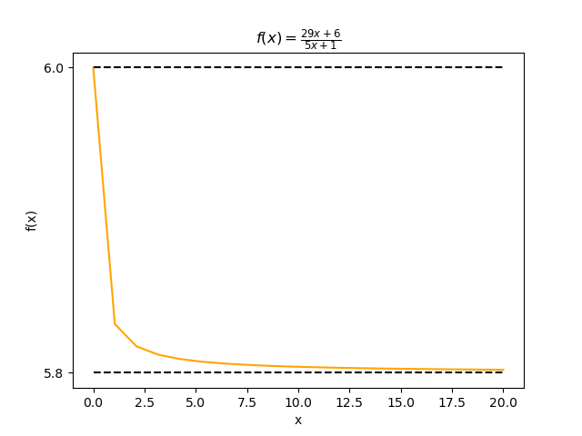
This means that \(f_3(x) = \frac{29x+6}{5x+1} = 5 + \frac{1}{\frac{5x+1}{4x+1}}\). Why is the quotient 5? Since \(\lim_{x \to 0} f_3(x) = 6\) and \(\lim_{x \to \infty} f_3(x) = \frac{29}{5} = 5.8\), the function is bounded by \(5.8 < f_3(x) < 6\) (note that \(0 < x < \infty\)). The quotient therefore has to be 5.

Now, we are ready to implement the symbolic form of the Euclidean algorithm by calling qr_matrix repeatedly:

def euclid_matrix_(m: np.ndarray) -> Iterator[Tuple[int, np.ndarray]]:
    """
    Symbolic Euclidean algorithm for a homographic function.

    :param m: The 2x2 matrix representing the function.
    :return: An iterator of the quotient and the remainder.
    """
    while True:
	if m[0][0] == 0 and m[0][1] == 0:
	    # if there is no remain, stop
	    break
	else:
	    (q, r) = qr_matrix(m)
	    if q is not None:
		yield q, r
		m = r
	    else:
		# if the quotient cannot be determined, stop
		break

Let's try it on \(\begin{bmatrix} 70 & 29 \\ 12 & 5 \end{bmatrix}\)

q = euclid_matrix_(np.array([[70, 29], [12, 5]]))
for (r, m) in q:
    pp_qr((r, m))
    print()

5 12  5
  10  4

1 10  4
   2  1

4  2  1
   2  0

So there is enough information in \(\frac{70x+29}{12x+5}\) to precisely determine 3 terms (5, 1, 4). The last matrix represents \(\frac{2x+1}{2x}\), an unbounded function. This means that depending on the next term of the input, the function can evaluate to any value. We don't have enough information to determine the quotient, so we have to stop.

As before, Gosper stacked the matrices in a compact format to illustrate the process:

print(euclid_matrix_tab(np.array([[70, 29], [12, 5]])))

70 29   
12  5  5
10  4  1
 2  1  4
 2  0   

This is a just an extension of the format that we use to visualize r2cf: we start with \(\begin{bmatrix} 70 & 29 \\ 12 & 5\end{bmatrix}\), end with \(\begin{bmatrix}2 & 1 \\ 2 & 0\end{bmatrix}\), and output 5, 1, 4 in the process.

Now, we can combine convergent calculation with the symbolic Euclidean algorithm. The first function below cf_transform_ returns the desired information (the quotient) along with internal states of the algorithm. It's useful for debugging and visualization. We use a second function cf_transform to filter out the internal states:

def cf_transform_(cf: Iterator[int], m0: np.ndarray = np.identity(2, int), finite_term = True) -> Iterator[Tuple[Optional[int], Optional[np.ndarray], np.ndarray, int, bool]]:
    """
    Transform a continued fraction.

    Exposes the internal states of the algorithm for visualization.
    A step can do: 1. Update the homographic matrix
		   2. Update, and an Euclidean step
		   3. Only an Euclidean step

    :param cf: The continued fraction.
    :param m0: The initial 2x2 matrix representing the transformatiom.
    :param finite-term: True, if cf is a continued fraction with finite terms.
			False, if cf represents a truncated continued fraction.
    :return: q: The quotient. None if the Euclidean step cannot be performed.
	     r: The remainder. None if the Euclidean step cannot be performed.
	     m: The 2x2 matrix before the Euclidean step
	     a: The term of the continued fraction that was used in this update
	     new_a: Was a new a term used?
		    False if this step only did Euclidean
    """
    m = m0
    for a in cf:
	m = np.matmul(m, h(a))
	new_a = True
	for (q, r) in euclid_matrix_(m):
	    yield q, r, m, a, new_a
	    new_a = False
	    m = r
	if new_a:
	    # Nothing was yielded.
	    # This convergent cannot be turned into a continued fraction
	    yield (None, None, m, a, new_a)

    # We will only reach this point if the series is finite
    if finite_term and m[1][0] != 0:
	for s in r2cf(Rational(m[0][0], m[1][0])):
	    yield s, None, m, a, False

def cf_transform(cf: Iterator[int], m0: np.ndarray = np.identity(2, int), finite_term = True) -> Iterator[int]:
    """
    Transform the input continued fraction into a new continued fraction.

    :param cf: The continued fraction.
    :param m0: The 2x2 matrix representing the transformation.
    :param finite_term: Is cf a finite-term fraction?
			Set to false if cf is a finite truncation of
			an infinite continued fractuon
    :return: A new continued fraction
    """
    for res in cf_transform_(cf, m0, finite_term):
	(q, r, m, a, new_a) = res
	if q is not None:
	    yield q
	else:
	    # q can be None, indicating that more terms are needed
	    # to continue. It can be ignored
	    pass

Run it on a continued fraction, and it just returns the same sequence. It doesn't seem to do any transformation. We'll see why the function is called cf_transform in the next section.

print(list(cf_transform(iter([2, 1, 1, 5, 1, 3]))))

[2, 1, 1, 5, 1, 3]

This seems to be anti-climatic for quite a bit of work… but here's something cool. Gosper combined the two stacked matrix representations that we have seen, to illustrate every step in the algorithm:

print(cf_transform_tab(iter([2, 1, 1, 5, 1, 3])))

  3 1 5 1 1 2    
        3 2 1 0  
      2 1 1 0 1 2
    6 1 1 0     1
  6 5 1 0       1
4 1 1 0         5
3 1 0           1
1 0             3

The numbers on the right are the outputs of cf_transform.

The beauty of the matrix representation is that we can transform convergents with a function of the form \(f(x) = \frac{px+q}{rx+s}\). All we need is an additional matrix multiplication on the left side! This can be calculated by giving cf_transform an initial matrix.

The continued fraction \([2, 1, 1, 5, 1]\) is \(\frac{33}{13}\). Let's double that, and turn it back to a continued fraction:

print("[2, 1, 1, 5, 1] is ", cf2r1(iter([2, 1, 1, 5, 1])))
print("The continued fraction of 66/13 is ", list(r2cf(Rational(66, 13))), "\n")
print(r2cf_tab(Rational(66, 13)))

[2, 1, 1, 5, 1] is  33/13
The continued fraction of 66/13 is  [5, 13] 

   66
   13   5   
    1   13  
    0

According to the above, \(2 * [2, 1, 1, 5, 1]\) is \([5, 13]\). How do we end up with fewer terms? We can illustrate the process by running cf_transform_tab with the initial matrix \(\begin{bmatrix} 2 & 0 \\ 0 & 1 \end{bmatrix}\) (which stands for the function \(f(x) = 2x\)):

m0 = np.array([[2, 0], [0, 1]], int)
cf = cf_transform(iter([2, 1, 1, 5, 1]), m0 = m0)
print(" 2 * [2, 1, 1, 5, 1] is ", list(cf), "\n")
print(cf_transform_tab(iter([2, 1, 1, 5, 1]), m0 = m0))

2 * [2, 1, 1, 5, 1] is  [5, 13] 

    1  5  1  1  2      
      10  6  4  2  0   
13 11  2  1  1  0  1  5
 1  1  0  1          13

Take one of the matrices in the tabulated display \(\begin{bmatrix} 6 & 4 \\ 1 & 1\end{bmatrix}\) for example. The range of \(\frac{6x+4}{x+1}\) is too wide (between 4 and 6) for the quotient to be determined. The algorithm therefore needs another term of the continued fraction. The matrix shifts leftwards without outputting a quotient. That's why the transformed continued fraction has a smaller number of terms.

Previously, we saw that the reciprocal of a continued fraction has an addition 0 in the beginning. Let's verify that with the initial matrix \(\begin{bmatrix} 0 & 1 \\ 1 & 0 \end{bmatrix}\) (which stands for the function \(f(x) = \frac{1}{x}\)):

m0 = np.array([[0, 1], [1, 0]], int)
cf = cf_transform(iter([2, 1, 1, 5, 1]), m0 = m0)
print("The reciprocal of [2, 1, 1, 5, 1] is ", list(cf), "\n")
print(cf_transform_tab(iter([2, 1, 1, 5, 1]), m0 = m0))

The reciprocal of [2, 1, 1, 5, 1] is  [0, 2, 1, 1, 5, 1] 

   1 5 1 1 2    
         1 0 1  
       3 2 1 0 0
     2 1 1 0   2
   6 1 1 0     1
 6 5 1 0       1
 1 1 0         5
 1 0           1

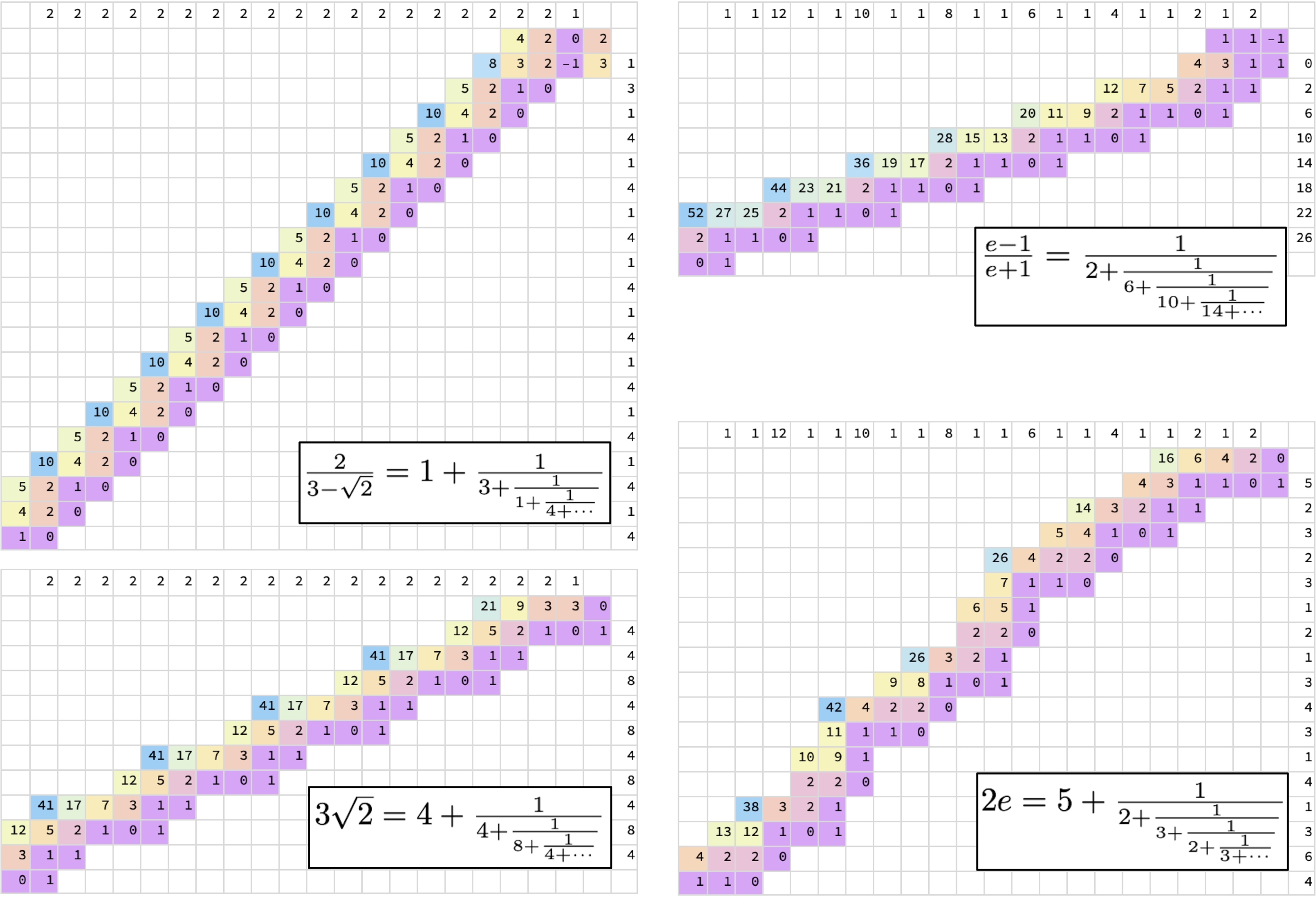
Another example: what is \(\frac{2}{3-\sqrt{2}}\) as a continued fraction? First, \(\sqrt{2} = [1, 2, 2, 2...]\), so we should define an infinite generator:

def cf_sqrt2():
    """A generator representing sqrt(2) as a continued fraction"""
    yield 1
    while True:
	yield 2

Then, we just need to run cf_transform with \(\begin{bmatrix} 0 & 2 \\ -1 & 3 \end{bmatrix}\) (which stands for \(\frac{2}{-x + 3}\)):

m0 = np.array([[0, 2], [-1, 3]], int)
cf = islice(cf_transform(cf_sqrt2(), m0 = m0), 6)
print(" 2 / (3 - sqrt(2)) is ", pp_inf_cf(list(cf)), "\n")
print(cf_transform_tab(islice(cf_sqrt2(), 6), m0 = m0))

2 / (3 - sqrt(2)) is  [1,3,1,4,1,4...] 

    2  2  2  2  2  1      
             4  2  0  2   
          8  3  2 -1  3  1
       5  2  1  0        3
   10  4  2  0           1
 5  2  1  0              4
 4  2  0                 1
 1  0                    4

The answer is a periodic continued fraction \([1, 3, 1, 4, 1, 4...]\).

Another example: what is \(\tanh{\frac{1}{2}} = \frac{e-1}{e+1}\)? We have already defined the continued fraction for \(e\), so it's just a matter of choosing the right initial matrix (\(\begin{bmatrix} 1 & -1 \\ 1 & 1 \end{bmatrix}\), representing \(\frac{x-1}{x+1}\)):

m0 = np.array([[1, -1], [1, 1]], int)
cf = islice(cf_transform(cf_e(), m0 = m0), 6)
print("(e-1)/(e+1) is ", pp_inf_cf(list(cf)), "\n")
print(cf_transform_tab(islice(cf_e(), 12), m0 = m0))

(e-1)/(e+1) is  [0,2,6,10,14,18...] 

     8  1  1  6  1  1  4  1  1  2  1  2      
                                   1  1 -1   
                                4  3  1  1  0
                      12  7  5  2  1  1     2
             20 11  9  2  1  1  0  1        6
    28 15 13  2  1  1  0  1                10
 17  2  1  1  0  1                         14
  1  0  1                                  17

The answer is a continued fraction with a simple pattern: after the second term, add 4 to the previous term.

I find the tabulated displays visually appealing, so I wrote some external codes (in Mathematica) to give them some colors. The colors make it easier to see the patterns in the numbers.

Before we proceed further, there is a small but important point that should be clarified. In the last example, we transformed \(e\) to calculate \(\frac{e-1}{e+1}\). It was done by truncating \(e\)'s infinite number of terms, retaining only the first 6 terms. This might give the impression that cf_transform is for approximating \(\frac{e-1}{e+1}\). That is not the case. The entire point of Gosper's work is to show that exact continued fraction arithmetic is possible. If this is not clear to you, let's define a different interface to cf_transform_, to make the point more obvious.

def cf_transform_func(cf: Iterator[int], m0: np.ndarray) -> Tuple[List[int], np.ndarray]:
    """
    Transform a continued continuation with finite number of terms.

    Returns a list (representing the transformed fraction) and the
    last homographic function so that it can be used on more terms.

    If cf is infinite, this function won't terminate.

    :param cf: The input continuned fraction.
    :param m0: A 2x2 matrix representing the transformation
    :return: A list representing the transformed fraction, and
	     a 2x2 matrix representing the homographic function
    """
    outputs: List[int] = []
    out_m: Optional[np.ndarray] = None
    for res in cf_transform_(cf, m0, finite_term = False):
	(q, r, m, a, new_a) = res
	if q is not None:
	    outputs = outputs + [q]
	    out_m = r
	else:
	    out_m = m
    assert isinstance(out_m, np.ndarray)
    return outputs, out_m

I call this function cf_transform_func, to emphasize that the output is a list integers, and a function represented by a matrix. The list of integers is an approximation, but together with the function, we have the exact solution to the computation. Why is it exact? Because if we have more terms of \(e\), we can send it to the function to get more output terms. This is a recursive process that can continue forever.

The example below, we call cf_transform_func with the first 6 terms of \(e\). We get 3 terms (0, 2, 6), and the function \(f(x) = \frac{9x + 2}{x}\), represented by the matrix. We can get 6 more terms of \(e\), and call cf_transform_func again with the matrix to continue the process.

m0 = np.array([[1, -1], [1, 1]], int)
cf = cf_e()
cf6 = islice(cf, 6)
(outs, m) = cf_transform_func(cf6, m0 = m0)
print("Using the first 6 terms of e, (e-1)/(e+1) is ", outs)
print("The homomorphic function is:\n ", m)
# take 6 more terms from e
cf6 = islice(cf, 6)
# we can continue our calculations to get more terms
(outs, m) = cf_transform_func(cf6, m0 = m)
print("With 6 more terms of e, we get ", outs)

Using the first 6 terms of e, (e-1)/(e+1) is  [0, 2, 6]
The homomorphic function is:
  [[9 2]
 [1 0]]
With 6 more terms of e, we get  [10, 14]

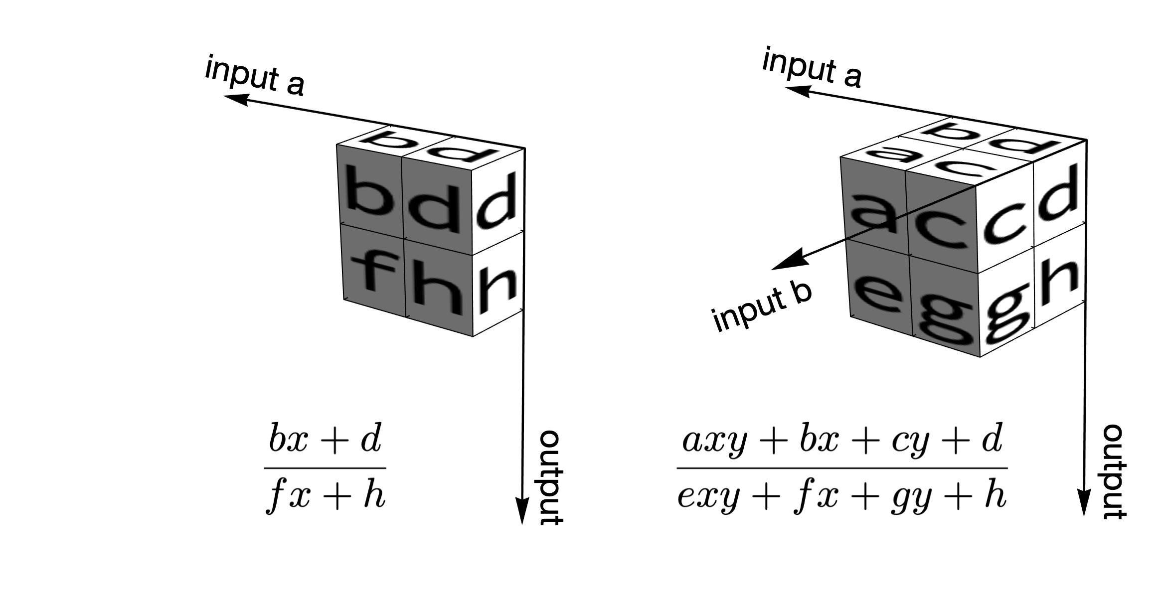
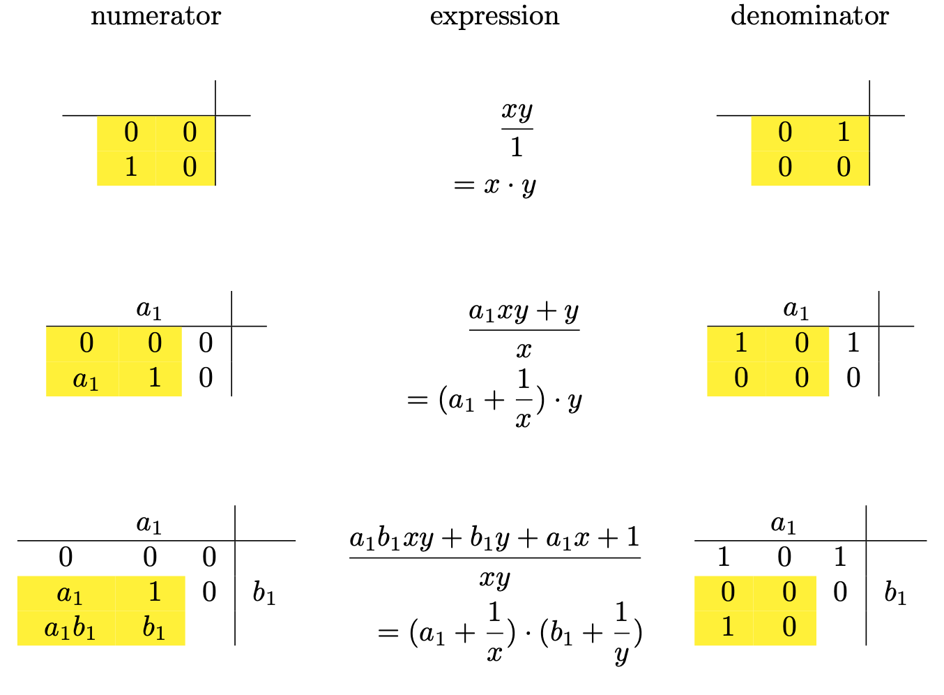
We have been dealing with one continued fraction at a time. In those situations, all operations involve functions of the form \(f(x) = \frac{px+q}{rx+s}\). They are known as homographic functions, and they can be represented by the matrix \(\begin{bmatrix} p & q \\ r & s \end{bmatrix}\). How do we generalize it to operations involving two continued fractions?

The problem is solved with bihomographic functions of the form \(f(x, y) = \frac{axy + bx + cy + d}{exy + fx + gy + h}\), where \(x\) and \(y\) are the unknown terms for the two continued fractions \(a\) and \(b\) respectively. We can write it in matrix form as:

Since we are working with two matrices as a single entity, it's natural to use tensors to represent bihomographic functions:

# Tensor representations of bihomographic functions

def tFrom2x4(m: np.ndarray) -> np.ndarray:
    """
    Translate a bihomographic function from algebraic to tensor form.

    :param m: A 2x4 matrix representing the function
    :return: A 2x2x2 tensor
    """
    ((a, b, c, d), (e, f, g, h)) = m.tolist()
    return np.array([[[b, d], [a, c]], [[f, h], [e, g]]])

def tTo2x4(m: np.ndarray) -> np.ndarray:
    """
    Translate a bihomographic function from tensor to algebraic form.

    :param m: A 2x2x2 tensor
    :return: A 2x4 matrix
    """

    (((b, d), (a, c)), ((f, h), (e, g))) = m.tolist()
    return np.array([[a, b, c, d], [e, f, g, h]])

I need a utility function to make it easy to access so many numbers in the tensors:

def tensor_ref(t: np.ndarray, label: str) -> Union[int, Tuple[int, int]]:
    """
    Easy accessing elements of a tensor

    :param t: A 2x2x2 tensor
    :param label: a-h refers to a number in the tensor
		  xy, x, y, 1 refers to numerator/denominator pairs
    :return: A number, or a pair of numbers
    """
    assert t.shape == (2, 2, 2)
    assert label in ['a', 'b', 'c', 'd', 'e', 'f', 'g', 'h', 'xy', 'x', 'y', '1']
    lookup = {}
    lookup['a']  = t[0,1,0]
    lookup['b']  = t[0,0,0]
    lookup['c']  = t[0,1,1]
    lookup['d']  = t[0,0,1]
    lookup['e']  = t[1,1,0]
    lookup['f']  = t[1,0,0]
    lookup['g']  = t[1,1,1]
    lookup['h']  = t[1,0,1]
    lookup['xy'] = lookup['a'], lookup['e']
    lookup['x']  = lookup['b'], lookup['f']
    lookup['y']  = lookup['c'], lookup['g']
    lookup['1']  = lookup['d'], lookup['h']
    return lookup[label]

What happens to \(f(x, y)\), with the addition of a new term \(a_n\) of \(a\)?

This is familiar, isn't it? It's exactly the same update rule that we use for updating the convergents! All we need to do is to right-multiply \(\begin{bmatrix} a_n & 1 \\ 1 & 0\end{bmatrix}\) the two matrices.

We can do the same with a new term \(b_n\) for \(b\):

This is basically the same thing, except that the direction is different. This corresponds to left-multiplying \(\begin{bmatrix} 0 & 1 \\ 1 & b_n\end{bmatrix}\).

The above suggests an elegant way to visualize continued fraction arithmetic: if we imagine that two matrices form a 2x2x2 cube, this cube moves leftwards upon receiving a new term of \(a\), and it moves downwards upon receiving a new term of \(b\). As before, we'll also use the Euclidean algorithm to convert the bihomographic function into continued fractions. When we get to perform the Euclidean step, the 2x2x2 cube moves in the third dimension. The following figure illustrates that continued fraction arithmetic is a direct generalization of the 2D case:

To implement the cube movements in Python, I use my favorite Numpy function: einsum (Einstein's sum; see this tutorial). If the very compact notation (invented by Einstein) seems cryptic, don't worry. It's just repeated matrix multiplication.

def apply_a(t: np.ndarray, a: int) -> np.ndarray:
    '''Move tensor t to the left by taking a new term of a'''
    ha = h(a)
    return np.einsum('dyx,xz->dyz', t, ha)

def h_rotated(b: int) -> np.ndarray:
    '''A rotated version of the 2x2 homgraphic matrix'''
    return np.array([[0, 1], [1, b]])

def apply_b(t: np.ndarray, b: int) -> np.ndarray:
    '''Move tensor t downwards by taking a new term of b'''
    hb = h_rotated(b)
    return np.einsum('zy,dyx->dzx', hb, t)

def apply_ab(t: np.ndarray, term: int, label: str) -> np.ndarray:
    """
    Apply a new term to the bihomographic tensor

    :param t: The tensor
    :param term: The new term to be applied to the tensor
    :param label: Is the term from continued fraction a or b?
    :return: A new 2x2x2 tensor
    """
    assert label in ['a', 'b']
    if label == 'a':
	return apply_a(t, term)
    else:
	return apply_b(t, term)

Something is curious about the discussion so far. We have a generic method for ingesting terms of two continued fractions, but how do we actually perform a specific operation on them? It's not hard to see that it all depends on the initial matrices. With appropriately chosen initial matrices, we can do multiplication, addition, division, subtraction, and their combinations. I think it's quite a remarkable result, because when we are dealing with numbers with multiple terms, multiplication is usually harder than addition. With continued fraction, the computational steps are exactly the same!

I made the following two figures to explain how addition and multiplication are done. Here's \(a+b\). We begin with just the initial matrices (first row), add the first term of \(a\), and then add the first term of \(b\).

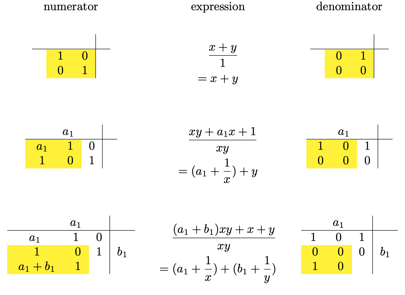
Here's the same process for multiplication:

These are the initial tensors for the four basic operations:

# Initial tensors for basic arithemtic operations

tForAddition = np.array([[[1, 0], [0, 1]], [[0, 1], [0, 0]]])
tForSubtraction = np.array([[[1, 0], [0, -1]], [[0, 1], [0, 0]]])
tForMultiplication = np.array([[[0, 0], [1, 0]], [[0, 1], [0, 0]]])
tForDivision = np.array([[[1, 0], [0, 0]], [[0, 0], [0, 1]]])

To make sure that the addition matrix works:

t = tForAddition
t = apply_ab(t, 2, 'a')
t = apply_ab(t, 3, 'b')
t = apply_ab(t, 4, 'a')
t = apply_ab(t, 5, 'b')
print(tTo2x4(t))

[[109  21  26   5]
 [ 20   4   5   1]]

\(\begin{bmatrix} 109 & 21 & 26 & 5 \\ 20 & 4 & 5 & 1 \end{bmatrix}\) means \(\frac{109xy + 21x + 26y + 5}{20xy + 4x + 5y + 1}\), which equals \((2+\frac{1}{4+\frac{1}{x}}) + (3+\frac{1}{5+\frac{1}{y}})\). That's correct.

Let's try multiplication:

t = tForMultiplication
t = apply_ab(t, 2, 'a')
t = apply_ab(t, 3, 'b')
t = apply_ab(t, 4, 'a')
print(tTo2x4(t))

[[27  9  6  2]
 [ 4  0  1  0]]

\(\frac{27xy+9x+6y+2}{4xy+y} = (2 + \frac{1}{4+\frac{1}{x}}) \cdot (3+\frac{1}{y})\). That's also correct.

By updating the bihomographic function with new terms of \(a\) and \(b\), we can generate a series of rational numbers that converges to the result. The following code does this by applying a new term of \(a\), and then a new term of \(b\)… and so on. This is not the only way to update the tensors. Any process that applies the terms in sequence will work. You can, for example, update with two terms of \(a\), and then two terms of \(b\).

# Continued fraction arithmethic - convergents

def arithmetic_convergents_(a: Iterator[int], b: Iterator[int], t0 = tForAddition) -> Iterator[Tuple[str, int, np.ndarray]]:
    """
    The convergents of doing arithemtic on two continued fractions.

    This version exposes the internal steps for visualization and debugging.
    New terms of the two continued fractions are applied alternately

    :param a: The first continued fraction.
    :param b: The second continued fraction.
    :param t0: The 2x2x2 tensor representing the operation.
    :return: The source (a or b?), the term, and the result (a 2x2x2 tensor)
    """
    res = t0.copy()
    while True:
	an = next(a, None)
	bn = next(b, None)

	if an is None and bn is None:
	    break

	if an is not None:
	    res = apply_ab(res, an, 'a')
	    yield 'a', an, res
	if bn is not None:
	    res = apply_ab(res, bn, 'b')
	    yield 'b', bn, res

def arithmetic_convergents(a: Iterator[int], b: Iterator[int], t0 = tForAddition) -> Iterator[Rational]:
    """
    The convergents of doing arithmetic on two continued fraction.

    This version returns an iteartor of rational numbers.
    :param a: The first continued fraction.
    :param b: The second continued fraction.
    :param t0: The 2x2x2 tensor representing the operation.
    :return: An iterator of rational numbers
    """
    c = arithmetic_convergents_(a, b, t0)
    for _, _, res in c:
	r = tensor_ref(res, 'xy')
	assert isinstance(r, tuple)
	yield Rational(r[0], r[1])

We have calculated previously that \(2*[2, 1, 1, 5, 1] = \frac{66}{13}\). Let's verify it by adding the continued fraction to itself:

a = iter([2, 1, 1, 5, 1])
b = iter([2, 1, 1, 5, 1])
print(list(arithmetic_convergents(a, b, tForAddition)))

[1/0, 4/1, 5/1, 6/1, 11/2, 20/4, 111/22, 616/121, 727/143, 858/169]

Yup. \(\frac{858}{169}\) equals to \(\frac{66}{13}\).

Let's try subtraction. Observe that \([2, 1, 1, 5, 1] - [2, 1, 1, 5, 1]\) does become 0 (that is \(\frac{0}{169}\)):

a = iter([2, 1, 1, 5, 1])
b = iter([2, 1, 1, 5, 1])
print(list(arithmetic_convergents(a, b, tForSubtraction)), "\n")

[-1/0, 0/1, 1/1, 0/1, -1/2, 0/4, 1/22, 0/121, -1/143, 0/169] 

Note that the numerator oscillates between -1, 0, and 1, while the denominator gets larger and larger.

How about division? Yup. \(\frac{429}{429}=1\).

a = iter([2, 1, 1, 5, 1])
b = iter([2, 1, 1, 5, 1])
print(list(arithmetic_convergents(a, b, tForDivision)), "\n")

[0/1, 2/2, 3/2, 3/3, 5/6, 10/10, 56/55, 308/308, 363/364, 429/429] 

Finally, let's try \(\sqrt{2}*\sqrt{2}\). With infinite number of terms, the answer should be 2. With finite number of terms, however, we get an approximation of 2 (\(\frac{9801}{4900}=2.0002\)).

a = islice(cf_sqrt2(), 6)
b = islice(cf_sqrt2(), 6)  
print(list(arithmetic_convergents(a, b, tForMultiplication)), "\n")

[1/0, 1/1, 3/2, 9/4, 21/10, 49/25, 119/60, 289/144, 697/348, 1681/841, 4059/2030, 9801/4900] 

Now we've come to visualization. Again, Gosper developed an ingenious method for visualizing the computational process, representing 2x2x2 tensors with a pseudo-3D effect. I decided not to implement his method because I find it hard to read. Instead, I will display the numerator and the denominator matrices separately. This format is not as compact as Gosper's method, but it works better when the numbers get large. In the figure below, the upper "band" is the evolution of the numerator matrix, and the lower band does the same for the denominator matrix. Note that for a 2x2 matrix in either band, you should read off the number in the lower-left corner, because \(\lim_{\substack{x\to \infty \\ y\to \infty}} \frac{axy + bx + cy + d}{exy + fx + gy + h} = \frac{a}{e}\).

a = iter([2, 1, 1, 5, 1])
b = iter([2, 1, 1, 5, 1])  
print(arithmetic_convergents_tab(a, b, tForAddition))  

      1   5   1   1   2        
                  2   1   0    
              1   1   0   1   2
          9   5   4   1       1
     61  11   6   5           1
131 111  20  11               5
727 616 111                   1
858 727                        
                  1   0   1    
              0   0   0   0    
          2   1   1   0        
     11   2   1   1            
 26  22   4   2                
143 121  22                    
169 143                        

The result \(\frac{858}{168}\) comes from the numbers at the lower-left corners of the two bands. Note that the row on top and the column on the right represent the two continued fractions.

Finally, some colors:

Unfortunately, I think these displays are not very satisfying, because the numbers tend to grow monotonically. That's because we haven't performed any Euclidean step. That's for the next section.

Since our tensors are just representations of bihomographic functions, it's straightforward to apply the Euclidean algorithm symbolically on them. euclid_tensor_ is almost identical to euclid_matrix_ in code structure:

# Continued fraction arithmetic - full version with Euclidean steps

def euclid_tensor_(t: np.ndarray) -> Iterator[Tuple[int, np.ndarray]]:
    """
    Symbolic Euclidean step for tensor t

    :param t: The 2x2x2 tensor
    :return: An iterator of quotient (an int) and remainder (a tensor)
    """
    while True:
	if np.all(t[0]==0):
	    # if the numerator is all zero, stop
	    break
	else:
	    (q, r) = qr_tensor(t)
	    if q is not None:
		yield q, r
		t = r
	    else:
		break

In the following example, we manage to extract three terms from the bihomographic function \(f(x, y) = \frac{3466xy + 1150x + 483y + 216}{1318xy + 601x + 182y + 83}\):

t = np.array([[[1550, 216], [3466, 483]], [[601, 83], [1318, 182]]])          
res = euclid_tensor_(t)
for (q, r) in res:
    print(q)

2
1
1

A tabulated format can be used to visualize the process. It is a generalization of the format that we used to visualize the symbolic Euclidean algorithm (see here), except that we are now flipping entire matrices instead of rows.

t = np.array([[[1550, 216], [3466, 483]], [[601, 83], [1318, 182]]])          
c = euclid_tensor_tab(t)
print(c)

1550  216     
3466  483     
 601   83    2
1318  182     
 348   50    1
 830  119     
 253   33    1
 488   63     
  95   17     
 342   56     

The algorithm stops after 3 steps, because the bihomographic function associated with the remainder of the last step \(f(x, y) = \frac{488xy+253x+63y+33}{342xy+95x+56y+17}\) is bounded by \(\frac{63}{56}=1.125\) and \(\frac{253}{95}=2.66316\). The range is too wide to determine a quotient.

Now it's time to combine the Euclidean algorithm (euclid_tensor_) with convergent calculation (arithmetic_convergents_). The code structure is basically the same as cf_transform_, except that there is one additional issue to consider: when we work with just one continued fraction, if the Euclidean step fails to determine a quotient, the only thing that we can do is to ingest one more term from the continued fraction. But now we have two continued fractions, so we have to decide which one to use. In terms of the 3D space, the question becomes: should we move the cube left or down? The decision is more or less arbitrary, because the Euclidean step will eventually sort out the result, as long as the terms from the two continued fractions are ingested sequentially. However, for visualization, we want to perform the Euclidean step as soon as possible, to prevent the numbers in the tensor from becoming too big. I use some heuristics from Gosper's paper to make this decision. The implementation (ABQueue) is in the Appendix.

def cf_arithmetic_(cf_a: Iterator[int], cf_b: Iterator[int], t0: np.ndarray, finite_term = True) -> Iterator:
    """
    Perform arithmetic operation on two continued fraction.

    :param cf_a: The first continued fraction.
    :param cf_b: The second continued fraction.
    :param t0: The 2x2x2 tensor representing the opertion.
    :param finite_term: Is this a finite-length continued fraction,
			or a truncation of an infinite one?
    :return: q - quotient (None if no Euclidean step performed)
	     r - remainder (2x2x2 tensor)
	     t - the tensor before the Euclidean step
	     term - the term used in the update
	     label - where does the term come from? cf_a or cf_b?
	     new_term - was a new term (either from cf_a or cf_b) used?
			It's false if only an Euclidean step was performed.
    """
    t = t0
    next_ab = ABQueue(cf_a, cf_b)

    while True:
	term, label = next_ab(t)
	if term is None and label is None:
	    # cf_a and cf_b are exhausted
	    break
	else:
	    assert isinstance(term, int)
	    assert isinstance(label, str)
	    t = apply_ab(t, term, label)
	    new_term = True
	    for (q, r) in euclid_tensor_(t):
		yield q, r, t, term, label, new_term
		t = r
		new_term = False
	    if new_term:
		# Nothing was yielded.
		# This means that an Euclidean step was not performed
		yield None, None, t, term, label, new_term

    # we will only reach this point if cf_a and cf_b have finite terms
    if finite_term and tensor_ref(t, 'e') != 0:
	rxy = tensor_ref(t, 'xy')
	assert isinstance(rxy, tuple)
	for s in r2cf(Rational(rxy[0], rxy[1])):
	    yield s, None, t, None, None, False
    else:
	# if the 'e' term is 0, that means the quotient is 0.
	# there is no need to return it
	pass

def cf_arithmetic(cf_a: Iterator[int], cf_b: Iterator[int], t0: np.ndarray, finite_term = True) -> Iterator[int]:
    """
    Perform arithmetic operation on two continued fractions.

    :param cf_a: The first continued fraction.
    :param cf_b: The second continued fraction.
    :param t0: The operation, represented by a 2x2x2 tensor.
    :param finite_term: Is this a continued fraction with finite terms,
			or a truncated one?
    :return: An iterator of the new continued fraction
    """
    for res in cf_arithmetic_(cf_a, cf_b, t0, finite_term = finite_term):
	(q, r, t, term, label, new_term) = res
	if q is not None:
	    yield q

def cf_arithmetic_func(cf_a: Iterator[int], cf_b: Iterator[int], t0: np.ndarray) -> Tuple[List[int], np.ndarray]:
    """
    Perform arithmetic operations on two finite-length continued fraction.

    Return a new fraction, and a bihomographic functiom, which can be
    applied to more terms.

    :param cf_a: The first finite-length continued fraction.
    :param cf_b: The second finite-length continued fraction.
    :param t0: A 2x2x2 tensor representing the operation.
    :return: A list, representing terms of the new continued fraction.
	     A 2x2x2 tensor representing the final bihomographic function.
    """
    outputs: List[int] = []
    out_t: Optional[np.ndarray] = None
    for res in cf_arithmetic_(cf_a, cf_b, t0, finite_term = False):
	q, r, t, term, label, new_term = res
	if q is not None:
	    outputs = outputs + [q]
	    out_t = r
	else:
	    out_t = t

    assert isinstance(out_t, np.ndarray)
    return outputs, out_t

In an earlier section, we showed that \(2 * [2, 1, 1, 5, 1] = [5, 13]\). Let's see if we can duplicate this by adding \([2, 1, 1, 5, 1]\) to itself.

a = iter([2, 1, 1, 5, 1])
b = iter([2, 1, 1, 5, 1])
print(list(cf_arithmetic(a, b, tForAddition)))

[5, 13]

It works! Subtraction?

a = iter([2, 1, 1, 5, 1])
b = iter([2, 1, 1, 5, 1])
print(list(cf_arithmetic(a, b, tForSubtraction)))

[0]

Yup! Multiplication?

a = iter([2, 1, 1, 5, 1])
b = iter([2, 1, 1, 5, 1])
print(list(cf_arithmetic(a, b, tForMultiplication)))

[6, 2, 3, 1, 18]

So, \(\Bigg( 2 + \frac{1}{1 + \frac{1}{1 + \frac{1}{5 + \frac{1}{1}}}} \Bigg)^2 = 6 + \frac{1}{2 + \frac{1}{3 + \frac{1}{1 + \frac{1}{18}}}}\). This is pretty cool, and it's something that we couldn't do before.

How about division?

a = iter([2, 1, 1, 5, 1])
b = iter([2, 1, 1, 5, 1])
print(list(cf_arithmetic(a, b, tForDivision)))

[1]

Also works. One more sanity check. This is a different way of demonstrating that the reciprocal of a continued fraction has an additional 0 in front. Note that the terms of a continued fraction are unique, except for the last one. \([2, 1, 1, 6]\) is just a different way of expressing \([2, 1, 1, 5, 1]\).

a = iter([1])
b = iter([2, 1, 1, 5, 1])
print(list(cf_arithmetic(a, b, tForDivision)))

[0, 2, 1, 1, 6]

Finally, a more difficult question: \(\sqrt{2} * \sqrt{2} = 2\). Because \(\sqrt{2}\) is an irrational number, we'll get 2 only if we have infinite number of terms. With finite number of terms, the best that we can do is approximation.

With 6 terms of \(\sqrt{2}\), we get \(2 + \frac{1}{4900}\)

a = islice(cf_sqrt2(), 6)
b = islice(cf_sqrt2(), 6)
print(list(cf_arithmetic(a, b, tForMultiplication)))

[2, 4900]

With 8 terms of \(\sqrt{2}\), we get \(2 + \frac{1}{5654884}\). So indeed, we are getting more accurate approximations of 2.

a = islice(cf_sqrt2(), 10)
b = islice(cf_sqrt2(), 10)
print(list(cf_arithmetic(a, b, tForMultiplication)))

[2, 5654884]

We don't have to truncate the inputs to finite terms. If the two continued fractions have infinite number of terms, we'll get the first term of the result (2) easily. However, if we ask for a second term, the program will get stuck in an infinite loop.

a = cf_sqrt2()
b = cf_sqrt2()
res = cf_arithmetic(a, b, tForMultiplication)
print(next(res))

2

Finally, we'll replicate a complex example in Gosper's paper. This example involves \(a=\frac{e^2+1}{e^2-1} = [1, 3, 5, 7\cdots]\), and \(b=\sqrt{6}=[2, 2, 4, 2, 4, 2\cdots]\). The goal is to calculate \(\frac{2ab+a}{ab+b}\).

First, define the two continued fractions:

def cf_sqrt6():
    """sqrt(6) = [2, 2, 4, 2, 4, 2...]"""
    yield 2
    yield 2
    while True:
	yield 4
	yield 2

def cf_coth1():
    """(e^2+1)/(e^2-1) = [1, 3, 5, 7...]"""
    s = 1
    while True:
	yield s
	s = s + 2

Then we calculate with cf_arithmettic:

t0 = np.array([[[1, 0], [2, 0]], [[0, 0], [1, 1]]])
b = islice(cf_sqrt6(), 4)
a = islice(cf_coth1(), 4)
c = cf_arithmetic(a, b, t0, finite_term = False)
print(list(c))

[1, 2, 1, 2, 1, 1]

Visualizing the process is much more difficult than the 2D cases. The tabulated display that I implemented is not very intuitive. It takes some time to learn to read it.

t0 = np.array([[[1, 0], [2, 0]], [[0, 0], [1, 1]]])
b = islice(cf_sqrt6(), 4)
a = islice(cf_coth1(), 4)
c = cf_arithmetic_tab(a, b, t0)
c.include_out = False
print(c)

        7    5    3    1          
                       1    0     
             8    2    2    0    2
            20    5    5    0     
                       0    0     
             7    2    1    1     
       74   14    4    2    2    2
      185   35   10               
             1    0               
       31    6    1               
       67   13    2              4
      299   58                    
       12    2                    
 366   51    9                    
1550  216   38                   2
3466  483                         
 116   16    4                    
 601   83   20                    
1318  182                         
 348   50                         
 830  119                         
 253   33                         
 488   63                         
  95   17                         
 342   56                         

This rendering should make it easier to understand what is going on:

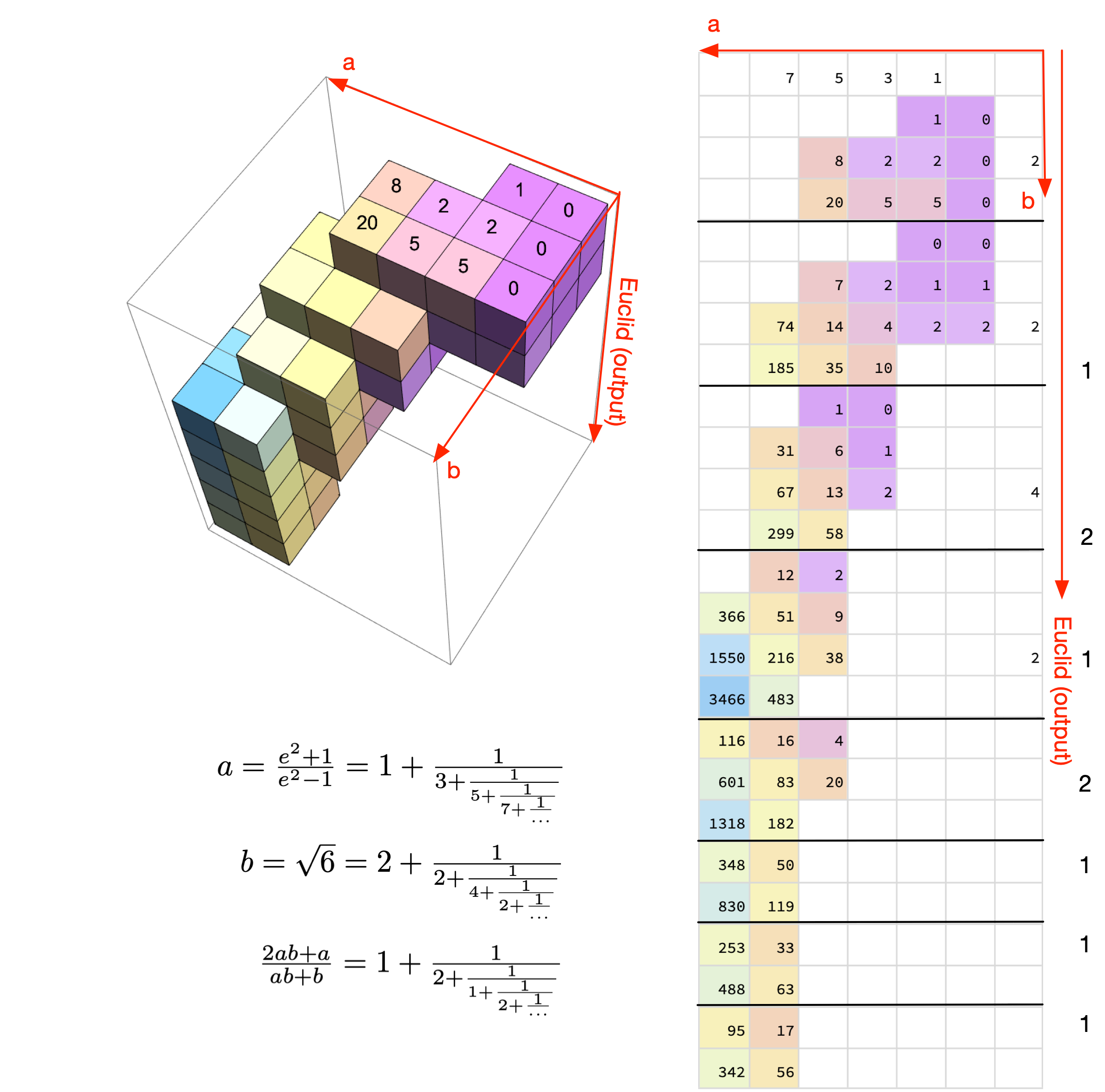
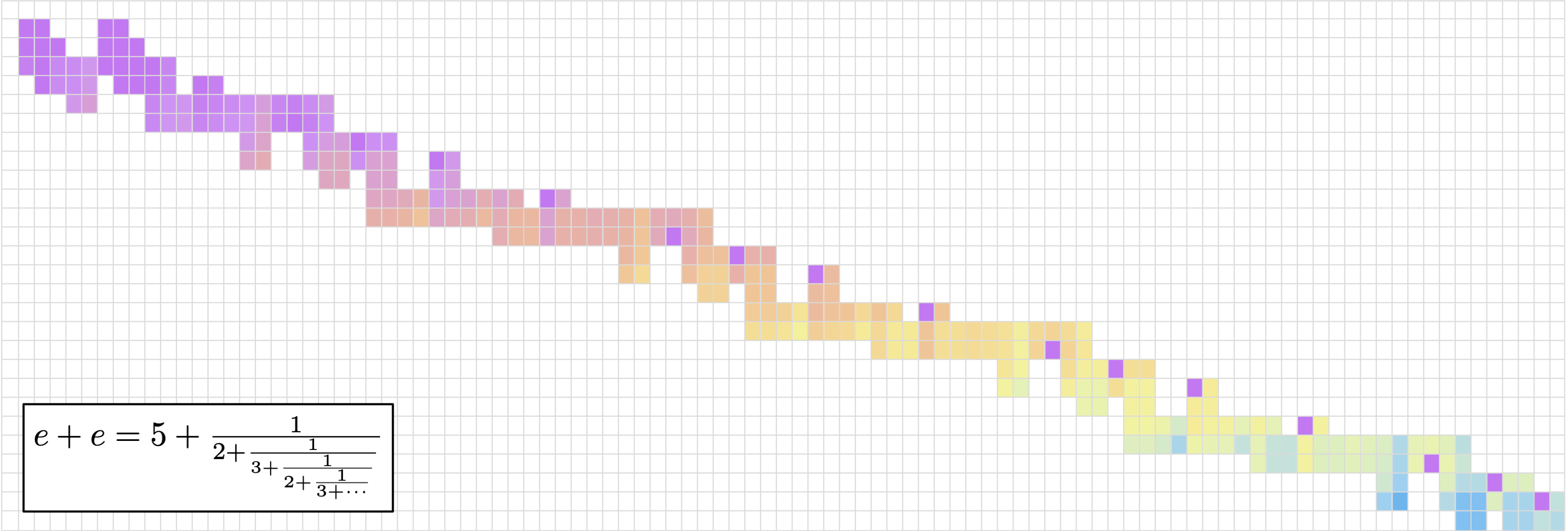
These images are fun to look at. Here's another one that I like. This is \(e+e=2e\). I rotated it to give it a horizontal orientation.

Given a homographic function represented by a 2x2 matrix, determine if the Euclidean step can be performed. If yes, return the quotient.

# Simple transformation of continued fraction

flip_m = np.array([[0, 1], [1, 0]])
identity_m = np.array([[1, 0], [0, 1]])

def flip_remain(m: np.ndarray, q: int) -> np.ndarray:
    """
    Caclulate the remainder, and then flip

    :param m: A 2x2 matrix
    :param q: The quotient
    :return: A 2x2 matrix
    """
    assert q >= 0, q
    r = m[0] - m[1] * q
    m[0] = r
    return np.matmul(flip_m, m)

def qr_matrix(m: np.ndarray) -> Tuple[Optional[int], np.ndarray]:
    """
    Calculate the quotient and the remainder of a 2x2 matrix

    :param m: A 2x2 matrix
    :return: The quotient (None if it cannot be found)
	     The remainder (2x2 matrix; idetity if quotient cannot be found)
    """

    assert not(m[1][0] == 0 and m[1][1] == 0)
    # This means that the series has already ended.
    # Nothing further needs to be done
    # The caller should not call qr_matrix in this case

    m2 = m.copy()

    if m2[1][0] == 0 or m2[1][1] == 0:
	# If the function is unbounded, the quotient cannot be determined
	return (None, identity_m)
    elif m2[1][1] < 0:
	# This means that the denominator can be made 0 (i.e., a singularity)
	return (None, identity_m)
    else:
	# If the function is bounded...
	v0: float = m[0][0] / m[1][0]
	v1: float = m[0][1] / m[1][1]
	v0, v1 = sorted([v0, v1])
	d0: int = math.floor(v0)
	d1: int = math.floor(v1)
	if d0 == d1:
	    # If d1 and d2 are the same, the quotient is determined
	    # Calculate the remain, and flip the matrix
	    m2 = flip_remain(m2, d1)
	    return d1, m2
	elif d1 == d0 + 1:
	    if d1 == v1:
		# This means that d1 is the upper-bound
		# it's only reached at 0 or infinity 
		# So d0 is the quotient
		m2 = flip_remain(m2, d0)
		return d0, m2
	    else:
		# The bounds are not tight enough to determine the quotient
		return (None, identity_m)
	else:
	    # The bounds are not tight enough to determine the quotient
	    return (None, identity_m)

This is the outline of the main code cont_frac.py.

<<IMPORTS>>
<<RATIONAL_NUM>>
<<R2CF>>
<<CONVERGENTS0>>
<<CONVERGENTS1>>
<<QR_MATRIX>>
<<CF_TRANSFORM>>
<<BIHOMOGRAPHY>>  
<<QR_TENSOR>>
<<ARITHMETIC>>
<<CF_EXAMPLES>>

def cf_pi():
    return iter([3, 7, 15, 1, 292, 1, 1, 1, 2, 1, 3, 1, 14, 2, 1, 1, 2, 2, 2, 2])

import math
import numpy as np
from typing import NamedTuple, Iterator, Tuple, Optional, Callable, Union, List

from cont_frac import *
from cont_frac_io import *
from itertools import islice